Structure of Systems - Mitochondrion Example

Introduction

In this document, we explore notations for representing the structure of systems – both at the macro level and at the micro level. Our background is in IT, so our main interest is in representing the structure of IT systems and their interfaces with human systems, business systems and other systems. However, we thought it would be useful to explore the problem, of structural representation, across a range of disciplines. We hope that we have acquired adequate knowledge, of these disciplines, to make the examples, taken from them, useful, but we certainly do not claim any deep knowledge of the disciplines. In this document, we take an example on the borderline between chemistry and biology, a mitochondrion organelle. We gradually introduce the concepts, of our approach to structural representation, as we develop this example. However, we first need to introduce some basic ideas.

Structure of Systems

What do we mean by a system? A system is any object that can contribute to change in either itself, or other systems. Biological systems, human systems, and business systems can ultimately be defined, as very complex compositions of chemical and physical systems. At the level of chemistry, systems are either quantities of energy or quantities of mass (i.e. atoms and electrons). At this level, within the universe, the total energy and the total mass are both conserved, i.e. both remain constant. At the level of nuclear chemistry, where radioactivity becomes relevant and there is seepage between mass and energy, we must take a broader view of mass, and recognise it as a form of energy, as given by the equation E=mc². With this broader definition of energy, within the universe, we still have conservation of energy (at least if we ignore black holes). Below the nuclear chemistry level, some physicists discuss the relationship, between energy and information, and take, as the fundamental concept, the conservation of information (thereby including black holes). In this document, we will use the term ‘system’ to encompass these different definitions.

When people talk of a system in the real world, they are usually imprecise. For instance, when we talk of the system, London, we may mean the ancient City of London, with its corporation and Lord Mayor, we may mean Greater London, with its more recently established mayor and councillors, we may mean London as a financial entity that is of concern to the City, we may be thinking of London as the capital of Great Britain (for now), we may include the people that live and work in London and the infrastructure that feeds into London. These are best thought of as different, though closely related, systems, with different, but overlapping, sets of component systems.

We should add a further observation, at this point. We need to recognise that there is an infinite number of systems, as any composition of a set of systems defines an additional system, even if its component systems are remote, totally unrelated, and never interact (i.e. never affect each other’s behaviour, directly or indirectly). Hence, we must concentrate our attention on “interesting” systems, each of which is composed of component systems that do interact, at some points in time.

When IT specialists represent the structure, of their systems, they usually make a strong distinction between the systems and the interfaces between these systems. We believe that this creates an artificial dichotomy, that constrains thinking, and becomes entrenched, in systems representations (e.g. with boxes and lines in diagrams). It also creates problems when different groups of engineers communicate – a simple interface, in a software engineer’s view of a system, expands into a complex hardware system, seen by a hardware engineer – the interfaces between chemical systems, as seen by chemists, expand into the complex physical systems, as seen by physicists. The fundamental concept, in our approach to structural representation, is the removal of the distinction between systems and interfaces. We see interfaces as being implemented by means of shared component systems.

Given our emphasis on shared component systems, we could, in theory, represent the structure of all systems, with a gigantic directed graph. The nodes, in the graph, would represent systems. A line, in the graph, would indicate that the system, that is represented at the bottom of the line, is a component of the system, that is represented at the top. The conservation rules, introduced above, mean that every system, considered as a collection of components, exists over all time, in some form, though it may be quiescent (not interacting) most of the time - the collection of atoms and energy, in Caesar’s last breath, though dispersed and transformed, still exists. Thus, our directed graph must remain static, representing the structure of all possible systems (including uninteresting ones), over all time. This leaves us with an important question – how is change represented?

In the real world, we see gradual change in systems. How does this gradual change relate to the static graph view, introduced above? The systems that are currently active (engaged in interactions) could be represented by an active subgraph, of our full directed graph. Most of the active graph will be in the lower, more detailed, levels of the full graph, as there reside the rapidly changing systems. The systems in the higher levels (as sets of direct component systems) change very slowly. This reflects reality - if you viewed a city or country very closely, you would see its detailed structure changing continually and rapidly, but if you viewed it from outer space, its visible, top-level, component structure would not appear to change.

The active subgraph gradually moves within the full graph. What triggers this movement? Proximity gives the clue – for elementary chemical systems, it is physical proximity that triggers an interaction (i.e. a chemical reaction). When close enough, the physical attraction of the protons of one chemical system, for the electrons of the other, is large enough to force a reconfiguration, of the electrons, and a binding, of the chemical systems. We need to generalise this concept of proximity. We believe that systems can only interact (in other words can only change each other), by means of shared component systems. This means that the interaction may be implemented in one of two ways. Either there might be a component system that is totally shared, between the two systems, or the two systems might both interact with a third system. These two forms of interaction provide our generalised understanding of proximity. Note that this is a recursive definition of an interaction – an interaction can only be activated, if all its component interactions can be activated, and this definition could nest down through many levels. Hence, it is primitive interactions, low in the directed graph, that implement those higher up. We referred to one primitive interaction above – the attraction between a proton, of one chemical system (an atom), and an electron, of the other – this attraction was a shared component between the two chemical systems.

In “Origin of the Species”, Darwin identified two orthogonal drivers for evolution -

• the continuous creation of new systems and
• the continuous disappearance of systems, as they were superseded by 'better' systems

Thus, in this document, we focus on a very small set of key concepts and assume a very, very, broad definition of the word, system – embracing anything that is involved in changes to other systems, including energy, atoms, cells, brains, IT systems, communication systems, businesses. We believe that all systems exist in a fractal-like structure - with each system being composed from a set of component systems – with each system only being able to interact with, and change other systems or be changed by them, if it shares component systems with the other systems - with a function being associable, with each shared component system, that defines that shared system’s effect on the sharing composite systems. We recognise that, even, with this sparse set of concepts, a system, in the real world, may be modelled in multiple ways, according to where one places the boundaries in the real-world. We have found that our set of concepts, although extremely sparse, still permits a very rich representation of (and even a full semantics for) systems and their evolution.

Our approach, to the representation of system structure, can be characterised as a lego-brick view of system structure, except that our bricks are more sophisticated in two ways. Firstly, our bricks can be built from smaller bricks. Secondly, the studs and recesses that connect our bricks can, also, be built from smaller bricks. Of course, here, the bricks and studs are the systems and interactions that we have been referring to, above.

Structural Representation of Mitochondrion

Levels of Abstraction

Throughout its seventy year history, the IT industry has seen, as its ideal, a top-down and evolutionary approach to systems design. Top-down involved starting with an abstract and undetailed view of the design (emphasising requirements), and then gradually working towards a less abstract and more detailed view (constrained by underlying systems). Top-down proved problematic, because it proved difficult to rigorously relate together the different levels of design. We believe that the strong and inflexible distinction between systems and their interfaces has been at the heart of this problem. This is our motivation for replacing the concept of interfaces with the concept of shared components.

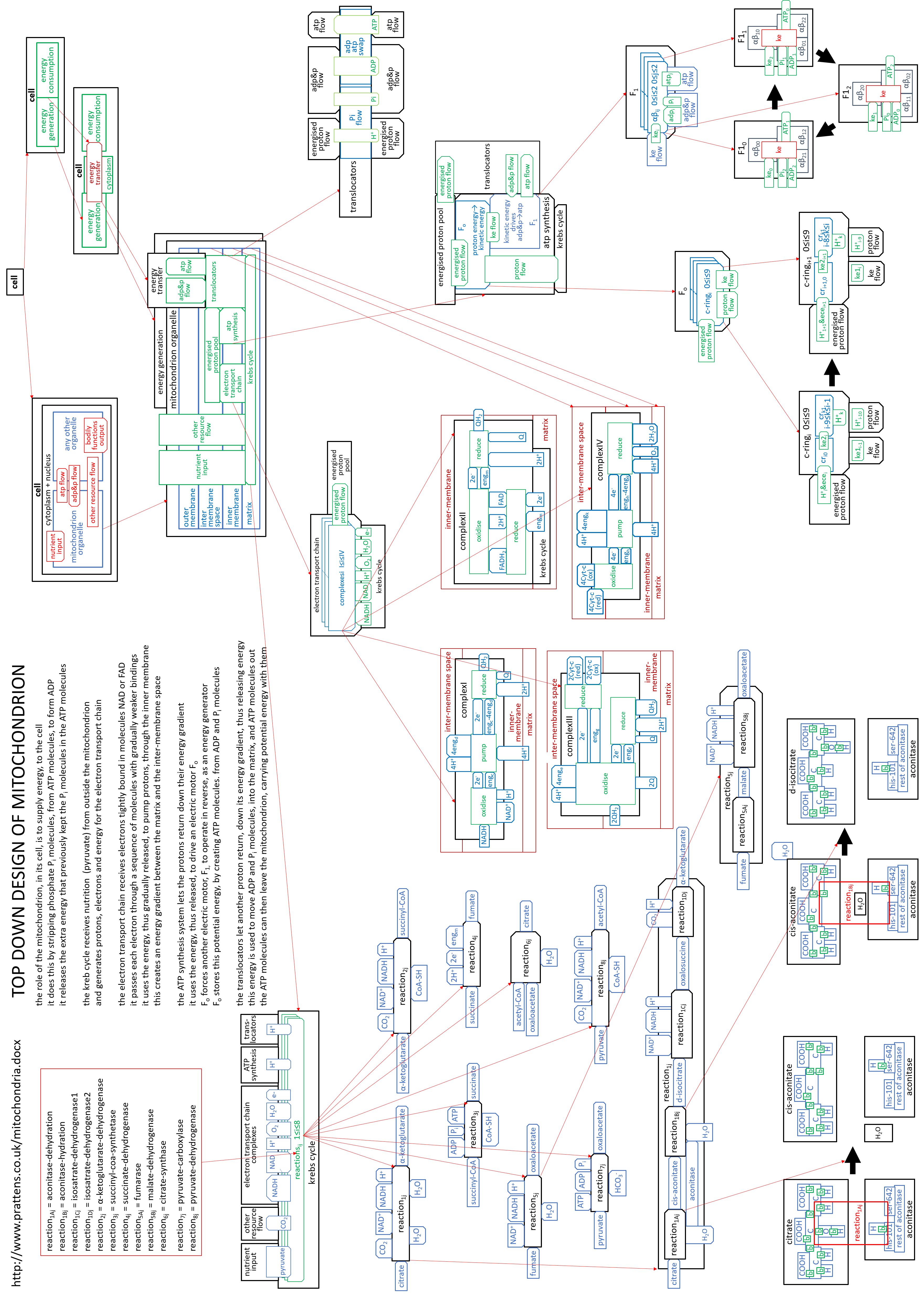
We cannot take a top-down approach to the design of a mitochondrion, because Darwinian evolution evolved the design billions of years ago. However, we can develop a top-down model of the mitochondrion. It might even indicate the steps taken in the Darwinian evolution.

We will develop our top-down model, of the mitochondrion organelle, passing through the following levels of abstraction:

• cell life cycle - at the highest level of abstraction, we have the cells (that contain mitochondria organelles) passing through their life cycles, with cells born, consuming other cells as food, generating new cells, and dying
• energy cycle - at the next level of abstraction, we can consider a mitochondrion organelle, as a consumer of food and a generator of energy, and the remaining organelles of the cell, as consumers of energy and generators of proteins, for use by other cells
• ADP/ATP cycle - at the next level, we can recognise that the mitochondria organelles store and transmit energy by converting ADP molecules into ATP molecules, and the other organelles release energy by converting ATP into ADP – thus using ATP molecules as carriers of potential energy (the currency of cells)
• proton cycle - the conversion of ADP to ATP requires energy and this is provided, in the form of electrochemical energy from a proton gradient (excess of protons and electrical charge), between the inner and outer layers of the mitochondrion organelle
• citric acid cycle - the Krebs, or citric-acid, cycle consumes the food that is received, by the mitochondrion, and uses it to provide protons, for the proton gradient
• free energy cycle - some chemical reactions generate surplus free energy and some require extra energy, before they can take place – these two sets of reactions need to be coupled, so that the former set can provide energy to the latter set, thus enabling them to jointly provide the chemical reactions that support the operations of the mitochondria (as outlined above)

Mitochondrion Organelle’s Role in the Cell

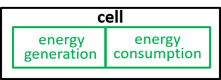
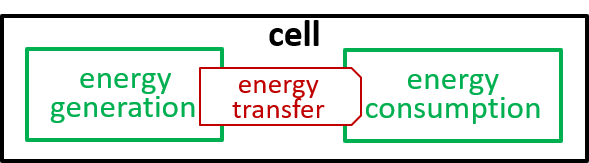
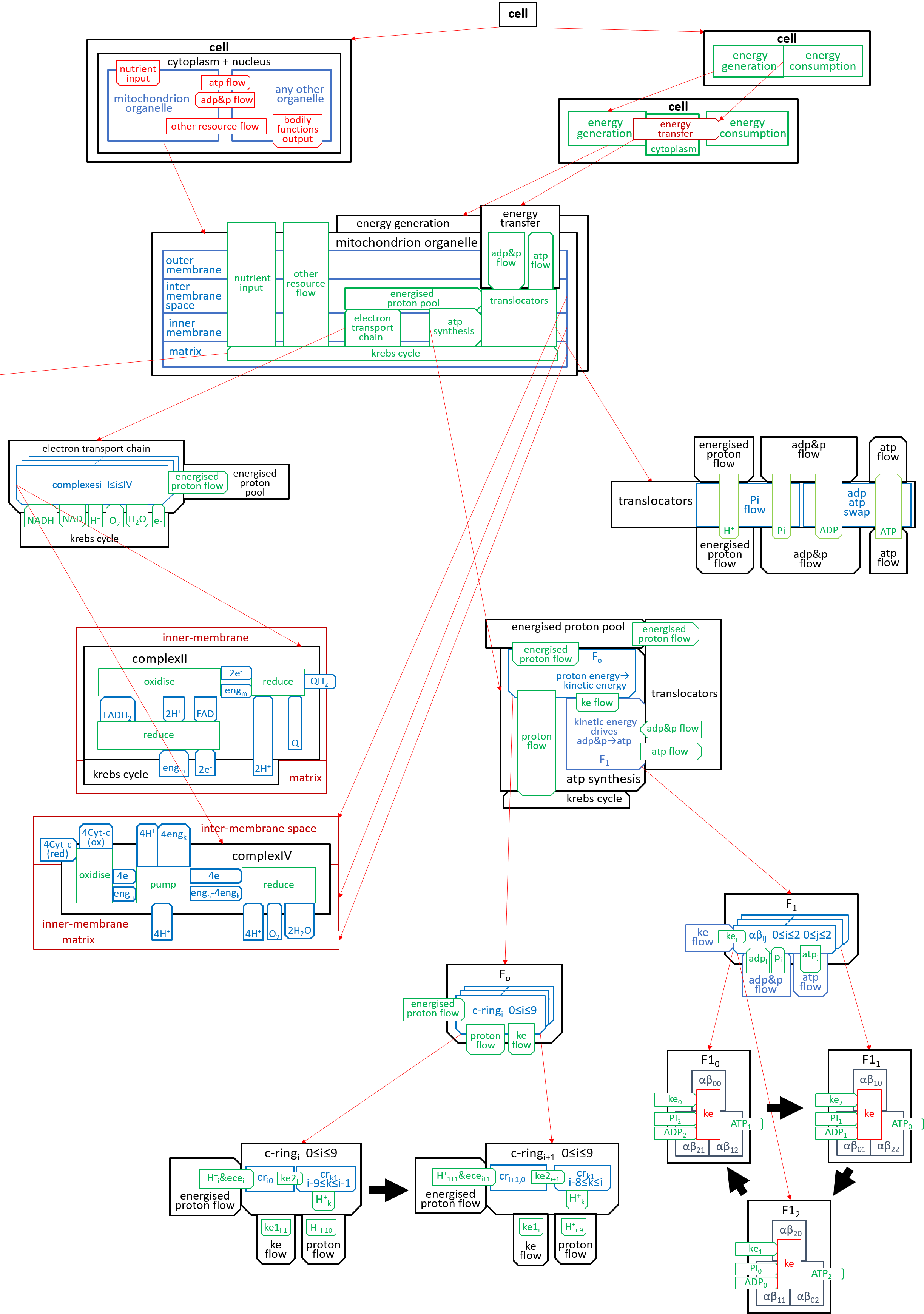
In our example, we consider the mitochondrion organelle only in its energy generation role. It has other roles, but we mostly ignore these. Hence, the starting point, for our example, could be a model of a cell, just from an energy generation and consumption point of view. To represent this, we can use either a directed graph or a lego-brick diagram: The dotted lines and the touching of the boxes indicate that there is some interaction, between the energy generation and energy consumption systems, but its nature is not known at present. This might be implemented in one of two ways. Either there might be a component system (e.g. energy transfer) that is totally shared between the energy generation and the energy consumption systems: or they might both interact with a third system (an extended energy transfer system) with the nature of these interactions unknown: Both pairs of diagrams could be valid. They could be considered as different views, as to where we set the boundaries, of the energy generation and consumption systems. The first pair sees the two systems (energy generation and consumption), as bigger systems (containing more components), than those seen in the second pair. This difference would only become apparent, when we developed more detailed diagrams. We referred to these different views of systems in the real world in our introductory sections.

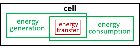
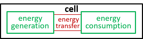
Ultimately, possibly at some very, very, low level in the directed graph, an interaction results in the transfer of component systems, across the boundary, between the interacting systems. We could show that the transfer is, predominantly, though not exclusively, in one direction, as shown. in the following diagrams. This extra decoration of the diagrams should only be viewed as guidance or clarification and not as definitive. There may be movement of component systems in both directions. The true nature, of the movement of component systems, should emerge later in more detailed diagrams.

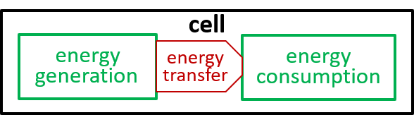
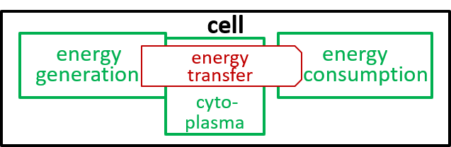
Acceptable alternatives for the last lego-brick diagram could be:

The presence of the cytoplasma component, in the second diagram, indicates that this component is involved in the energy transfer interaction.

We could encounter systems that combine component systems in ways that are, so complex, that it is impossible to represent them in lego-brick diagrams. We can normally get around this problem, by developing our representation, in small steps - we do this, in this document. We could, also, get around the problem, by providing textual equivalents, of the diagrams. For instance, a textual equivalent, of the above diagram, is:

α:cl{ β:eg{ε:int}, γ:et{ε,ζ}, δ:ec{ζ:int} }

cl=cell eg=energy-generation et=energy-transfer ec=energy-consumption int=interaction

We only really need the Greek letters for the components that are shared, so can simplify the above to:

cl{ eg{α:int}, et{α,β}, ec{β:int} }

cl=cell eg=energy-generation et=energy-transfer ec=energy-consumption int=some-interaction

Molecules act as containers of potential energy. Energy is required to combine atoms, or molecules, in molecules. The energy is released when the molecule is split into its component atoms, or molecules. This storage and release of energy is exploited, by a cell, in its ATP/ADP cycle

An APT molecule contains three component phosphate molecules, while an ADP molecule contains only two. A mitochondrion organelle, in a cell, uses energy to add one phosphate molecule (Pi) to ADP, to create ATP. Other organelles, in the cell, release (and use) the energy by removing one phosphate molecule from ATP, to create ADP. We can represent this with:

cl{ cy{mo{ α:at, β:ad, γ:or, δ }, oo{ α, β, γ, ε }, δ:ni, ε:bf } } cl=cell cy=cytoplasm mo=mitochondrion oo=any-other-organelle int=interaction ni=nutrient at=atp-flow ad=adp&p-flow or=other-resource bf=bodily-function

The directed graph, the textual description and the lego-brick diagram should, each, tell us how to draw and/or write the other two.

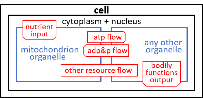
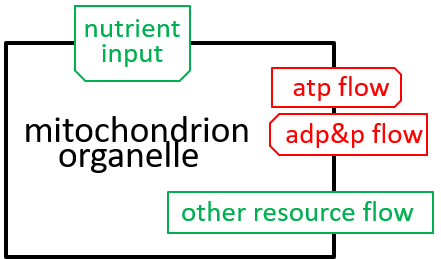
The cell takes in nutrients and supports the various functions of the body that contains the cell. The ADP/ATP cycle transfers energy from mitochondrion organelle to other organelles. The other resources, shown, are detailed, in the next section.

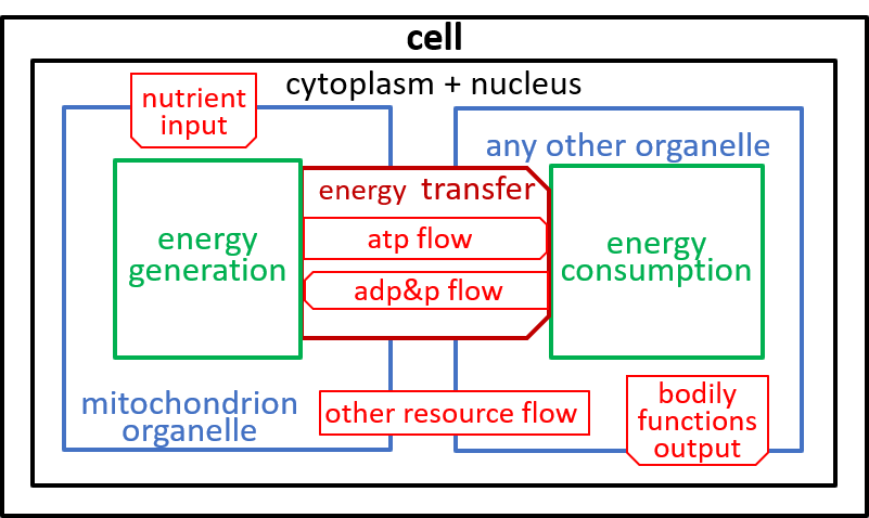
The relationship, between this diagram and earlier diagrams, can be represented by:

cl{ cy{ mo{ α, γ:or, eg{ε,ζ:int}, δ:et{at{ε,ζ},ad{ζ,θ}} }, oo{ β, γ, ec{η,θ:int}, δ }, α:ni, β:bf } } cl=cell cy=cytoplasm mo=mitochondrion oo=any-other-organelle int=interaction eg=energy-generation ec=energy-consumption et=energy-transfer ni=nutrient at=atp-flow ad=adp&p-flow or=other-resource bf=bodily-function

Component Structure of the Mitochondrion Organelle

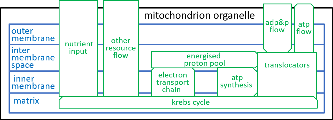
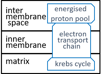
We are, now, in a position to explore the detailed structure of the mitochondrion organelle as shown in our earlier diagram (and repeated here):

and take it to the next levels of detail:

mo{ om{ α, β, γ, δ }, is{ α, β, ε:et{σ,τ:int}, ζ:pp{σ, ς,υ:int}, η:as{ς, π,ρ:int }, θ:tr{υ,π, χ,φ,ξ:int }, γ:ad{χ}, δ:at{φ} } im{ α,β,ε,η,θ }, ma{ α:ni{ω:int}, β:or;{ψ:int}, ε,η,θ, λ:kc{ω,ψ,τ,ρ,ξ} } } mo=mitochondrion, om=outer-membrane, is=inter-membrane-space, im=inner-membrane, ma=matrix ni=nutrient at=atp-flow ad=adp&p-flow or=other-resource kc=krebs-cycle et=electron-transport pp=energised-proton-pool as=atp-synthesis tr=translocators int=interaction

It is very important to realise that this diagram (like our earlier diagrams) does not attempt to represent physical layout. Physically, in three-dimensional Euclidean space, the mitochondrion has two concentric membranes, or skins, its inner-membrane and its outer-membrane. The space, within the inner-membrane, is called the matrix, and the space, between the two membranes, is called the inter-membrane space. Hence, physically the matrix is within the inner-membrane, but it is, not, in our model, a component system of the inner-membrane. The above diagram (and its equivalent directed graph and textual description) represent the component structure, of the mitochondrion organelle – how it is composed, from component systems.

From an energy point of view, the most important component system of the mitochondrion organelle is the ATP synthesis system. It is responsible, for the conversion of ADP molecules into ATP molecules. As we indicated above, this is the mechanism, by which the mitochondrion organelle stores and transmits energy, for use by other organelles.

The electron-transport-chain creates and maintains a proton-gradient (an excess of protons (H⁺s) and hence an excess of electro-chemical energy) between the inter-membrane space and the matrix. This enables it to continually deliver electro-chemical energy to drive the ATP synthesis system,

The inner-membrane is impermeable to all chemicals other than O₂, CO₂, and H₂O. However, the mitochondrion needs to transfer NADH, NAD⁺, ADP, ATP, and H⁺ between its inter-membrane space and its matrix. It achieves this with special component systems that exist within the inner-membrane – translocators (as well as shuttles and antiports).

The Krebs Cycle receives food (e.g. glucose), from outside the mitochondrion, and generates the resources that are needed, by the other component systems of the mitochondrion.

In the following subsections we will give detailed representations of these components.

The ATP Synthesis Motors

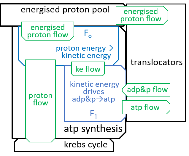
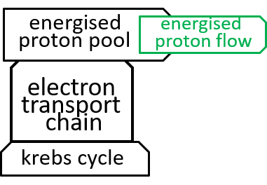
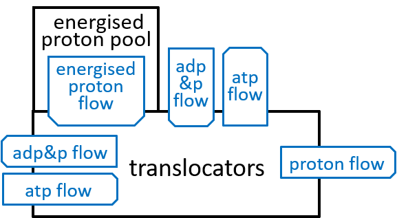
Remember that we said, in an earlier section, that the inner-membrane of the mitochondrion is impermeable to protons. The electron transport chain and the ATP-synthesis component systems provide routes through this impermeableness. The first, the electron transport chain, forces protons through the inner-membrane, from the matrix to the inter-membrane space, so that there are more protons in the latter than the former, thus forming a proton gradient that effectively gives electro-chemical energy to the protons. The second, the ATP synthesis system, allows the energised protons to flow, in the opposite direction, down this gradient, and uses the electro-chemical energy that is released to perform its ATP synthesis role. The proton gradient is thus analogous (with protons, rather than water) to the huge hydro-powered ‘battery’ system, at Elidir Mountain, in Wales. Darwinian evolution invented such batteries (miniaturised and highly efficient) billions of years ago.

In the diagram, at the end of the previous section, the ATP synthesis system was represented with: We can now expand ATP synthesis to give: The ATP synthesis system is a very complex chemical structure. However, it effectively functions as two motors, which the chemists have simply named, F_o and F₁. One of these motors, F_o, is an electric motor, driven by the electro-chemical potential of the protons, as they flow down the proton gradient. This F_o motor is embedded in the inner-membrane, but it has a rotating spindle that extends into the matrix. It converts the electro-chemical energy that it releases from the protons into the kinetic energy of the rotating spindle. The other motor, F₁, is contained in the matrix and could, potentially, be driven by the chemical energy stored in ATP and could also produce kinetic energy, to drive the spindle. In fact, within the ATP synthesis system, this motor is forced, by the spindle of the other motor, to work in reverse mode, operating as a generator of ATP, using kinetic energy to create ATP from ADP and Pi. We have described this pair of motors, in this way, because they can operate in reverse and they do just that when necessary. It seems that, billions of years before Faraday was born, Darwinian-evolution evolved the electro-chemical motors, F_o and F₁, and copied them, into most living cells.

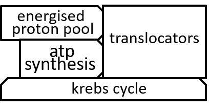
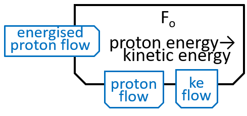
The F_o motor was shown in the last diagram with: Ten protons need to flow, down through F_o, in order to rotate the spindle (referred to above) through 360° and return it to its initial state. F_o passes through ten states, as the ten protons gradually flow through it. In each state, one proton is being released, from F_o into F₁, eight protons remain held in F_o, and another proton is being acquired (from the energised proton flow).

The main component, of the F_o system, is the c-ring, a ring of 10 subunits, each containing a chemical (Asp61) that can absorb a proton. The c-ring also has the spindle, attached at its centre and extending into F₁. Each proton enters the c-ring and is absorbed into the adjacent subunit. This changes the shape, of the subunit, and forces a rotation by 36°, of the c-ring, thus giving kinetic energy to the spindle. The proton is released when the ring has rotated a further 324° (9x36°), and thus makes its subunit available for a later proton.

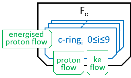
We can name the subunits cr_i with 0≤i≤9. The labels, i, should be treated as numbers modulo 10. When we look at a non-digital clock face, we see numbers modulo 12. If the clock tells you that that you fell asleep at 10 o-clock and awoke at 6-oclock, then you will know that you have been asleep 8 hours. Likewise, with numbers modulo 10, if i is 6, then i-9 should be understood as 7.

Thus, the c-ring has ten states c-ring_i with 0≤i≤9: We can see that each subunit, cr_i, has two states, which we can name as cr_i1 (with proton absorbed) and cr_i0 (without proton). Then, each of the 10 states of the c-ring is equivalent to states of its subunits, as defined by:
c-ring_i = { cr_i,0, cr_i-1,1, cr_i-2,1, cr_i-3,1, cr_i-4,1, cr_i-5,1, cr_i-6,1, cr_i-7,1, cr_i-8,1, cr_i-9,1 } with 0≤i≤9.

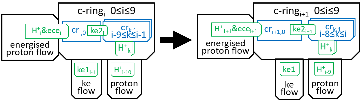
We now need to consider the transitions between successive states of the c-ring. At a simple level we can represent the transitions by:

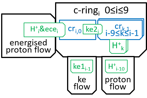
Within the c-ring, as the proton moves from inter-membrane space to matrix, it loses its electro-chemical energy (ece_i). Some of this energy is used in absorbing the proton H⁺_i, into subunit cr_i0, to create cr_i1. The rest is transformed into kinetic energy. Some of this kinetic energy (ke1_i) is used to rotate the spindle through 36°, thus transmitting energy to F₁. Some (ke2_i) is used, by the subunits of the c-ring, to push the rest of the subunits round the spindle (reflecting the fact that the subunits are in immediate proximity, to each other). We said in the introductory sections that an interaction between two systems could only take place by means of shared components and the functions they perform. It is the electro-chemical energy ece_i that drives the interaction. The interaction can be represented, textually, at a high level of detail, with a function:

ece_i( { epf_i, crg_i, kef_i, pfl_i } ) = { epf_i+1, crg_i+1, kef_i+1, pfl_i+1 }

ece_i( { epf_i{ α_i+1, β_i:H⁺_i, γ_i:ece_i }, crg_i{ β_i, γ_i, δ_i:cr_i0{ζ_i:ke2_i}, { ε_k:cr_k1{ζ_k, η_k:int}, β_k:H⁺_k{η_k} }_{i-9≤k≤i-1} },

            θ_i-1:kef_i-1{ kel_i-1, kef_i-2 }, κ_i-10:pfl_i-10{ H⁺_i-10, pfl_i-11 } } )

= { α_i+1:epf_i+1{ epf_i+2, β_i+1:H⁺_i+1, γ_i+1:ece_i+1 }, crg_i+1{ β_i+1, γ_i+1, cr_i+1,0{ζ_i+1:ke2_i+2}, {ε_k}_i-8≤k≤i },

       kef_i{ ke1_i, θ_i-1 }, pfl_i-9{ H⁺_i-9, κ_i-10 } }

ece=electro-chemical-energy epf=energised-proton-flow crg=c-ring kef=kinetic-energy-flow pfl=proton-flow

H+=proton cr=c-ring-subunit ke=kinetic-energy

It is clear, from the above example, that the textual representation is harder, for the reader, to understand, than the diagrammatic representation. However, the textual representation does open-up the possibility, of simulating the systems that are represented.

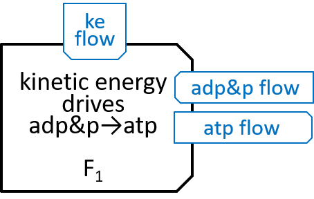
The F_o system was comparatively simple, in that it just had 10 similar states. The F₁ system is a bit more complicated. It was represented above with:

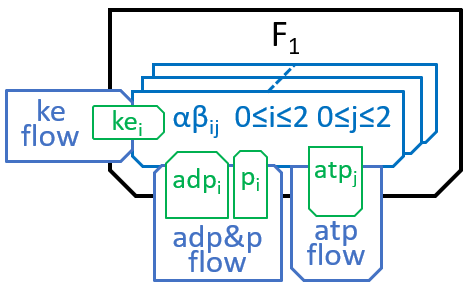
F₁ has a ring, containing three identical pairs of proteins, the pair of proteins that chemists refer to as α and β. Each of the αβ pairs (labelled αβ_i with i=0,1 and 2) cycles through three states (labelled αβ_ij, with j=0,1 and 2 for each i):

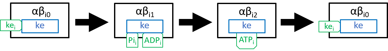
In state j=0, an αβ_i pair has nothing attached; in state j=1 it has ADP and Pi molecules attached; and in state j=2 it has an ATP molecule attached. The transition, between states j=0 and j=1, attaches ADP and Pi molecules; the transition, between states j=1 and j=2, uses kinetic energy to force the ADP and Pi molecules together and, thus, forms an ATP molecule; the transition between states j=2 and j=0 detaches the ATP molecule, as in:

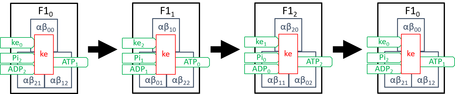
We need to explain the component, ke. Firstly, it drives each αβ_i pairs (0=i=2) through the three states αβ_ik\ pairs (0=k=2), described above. Secondly, it ensures that the three αβ_i pairs (0=i=2) are constrained to always be at different states, in their cycles. The rotation of the spindle provides most of the kinetic energy. However, the reconfiguration of each αβ_i pair, when forcing ADP and Pi molecules together, also has kinetic effect on neighbouring αβ_i pairs. It may be that the second source suffices to achieve the second aim, mentioned above. However, we believe that this is still a subject for debate, amongst researchers. The transitions between the three states of F₁ (labelled F1_i, with 0=i=2) can be represented by:

ke({ F1i{ α:ABi,0{ δ:kei, ε:ke }, β:ABi+2,1{ ε, ζ:Pii+2, η:ADPi+2 }, γ:ABi+1,2{ ε, θ:ATPi+1 } }, κ:Pii, λ:ADPi, μ:kei+1 }) = { F1i+1{ γ{ μ, ε }, α{ κ, λ, ε }, β{ ATPi+2{ ζ, η }, ε } }, θ } mo=mitochondrion, om=outer-membrane, is=inter-membrane-space, im=inner-membrane, ma=matrix ni=nutrient at=atp-flow ad=adp&p-flow or=other-resource kc=krebs-cycle et=electron-transport pp=energised-proton-pool as=atp-synthesis tr=translocators int=interaction

For convenience of drawing the diagram, we have shown the three αβ_i pairs rotating 120° anticlockwise with each transition. They also rotate physically, but it is not our purpose to represent the physical movement. We have also written AB for αβ, in our textual representation. This is because, we have reserved lower case Greek letters as local identifiers. As we said for F_o, we would like to model F₁, in more detail, but we are stopped firstly, by our uncertainty about the exact use of the kinetic energy in the transformations and secondly, by our believe that the chemists have yet to agree some details.

Given the above descriptions of F₁ and F_o, one would expect F_o to require 9 (or some multiple of 3) protons and their associated electro-chemical energy, to drive each 360° rotation, of the spindle. In fact, chemists believe it receives 10. We understand that research, on F_o, is still underway, but it is believed that more than 3 protons (approximately 3.33) are required to provide enough energy, for the generation of each ATP molecule. Furthermore, this quantity may vary slightly, with variations in the energy gradient between the inter-membrane space and the matrix.

The Electron Transport Chain

Earlier diagrams have represented the Electron Transport Chain with:

The role, of the Electron Transport Chain, is to maintain the proton gradient, needed by the ATP synthesis system, and described, in the previous section. To do this, it must pump protons, through the inner membrane. This requires energy. The energy is obtained, by moving electrons, between molecules, with an oxidation reaction releasing an electron, from a donor molecule, and a reduction reaction acquiring the electron, for an acceptor molecule. This works, because, in the Electron Transport Chain, the donor molecules chosen (by Darwinian evolution) hold their electrons in higher-energy grips than the acceptor molecules. The spare energy, thus released, can be used, to pump protons, up the gradient, from matrix to inter-membrane space.

Electrons are only free for a very short time, so an oxidation reaction is always quickly followed by a reduction reaction, thus combining the two reactions in a redox reaction. The pairings:

	NADH→NAD++2e-+H+	and	Q+2e-+2H+→QH2
	QH2→Q+2e-+2H+	and	cyt-c(oxigenated)+e-→cyt-c(reduced)
	cyt-c(reduced)→cyt-c(oxigenated)+e-	and	O2+4e-+4H+→2H2O

provide the redox reactions of the Electron Transport Chain. Electrons move down the chain - NAD → Q → cyt-c → O₂ - with each link in the chain having a weaker hold on its electrons than its predecessor. The three chemical systems that perform the three redox reactions are referred to as Complex I, Complex III, and Complex IV.

There is a subsidiary path, performed by Complex II, that replaces the first pair with:

FADH2→FAD+2e-+2H+

and

Q+2e-+2H+→QH2

At first sight, the name Electron Transport Chain may seem peculiar, as the purpose of the system, so named, is to transfer protons, from the matrix to the inter-membrane space. However, these transfers require energy, and this energy is released, by the movements, of electrons, through the Electron Transport Chain.

We could ask, why has Darwinian Evolution evolved four steps, when it could have used one step, involving just NAD and O2. The answer is that the one step would have been too explosive, releasing a large amount of energy, most of which would have been dissipated as heat. Darwinian Evolution evolved four steps, so that the spare energy could be released slowly, in manageable quantities.

The, above, four steps, of the Electron Transport Chain, differ in their details, but are similar in their essentials. The following shows what they have in common (remember that oxidising removes an electron (thus increases charge) and reduction adds it (thus reducing charge)):

e-=electron eng=energy

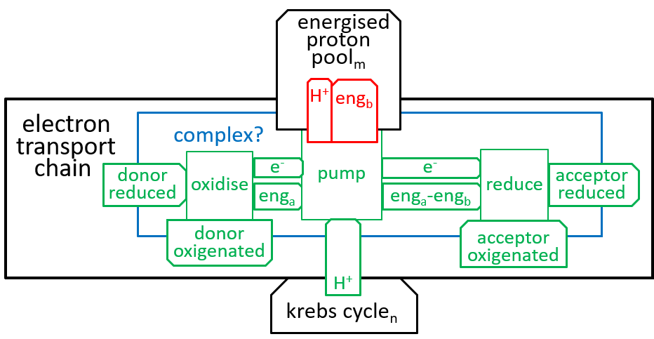
The states of the energised proton pool and the krebs cycle systems are both dependent on the number of protons that they contain. The state labels m and n represent these numbers. Each of the five Complexes increases m and decreases n; the ATP Synthesis system does the opposite. enga is the energy that is released by the oxidisation. engb is the electro-chemical energy acquired by a proton, when moved from matrix to the inter-membrane space. engb can vary a bit, depending on the number of protons (n), in the matrix, relative to the number (m), in the inter-membrane space.

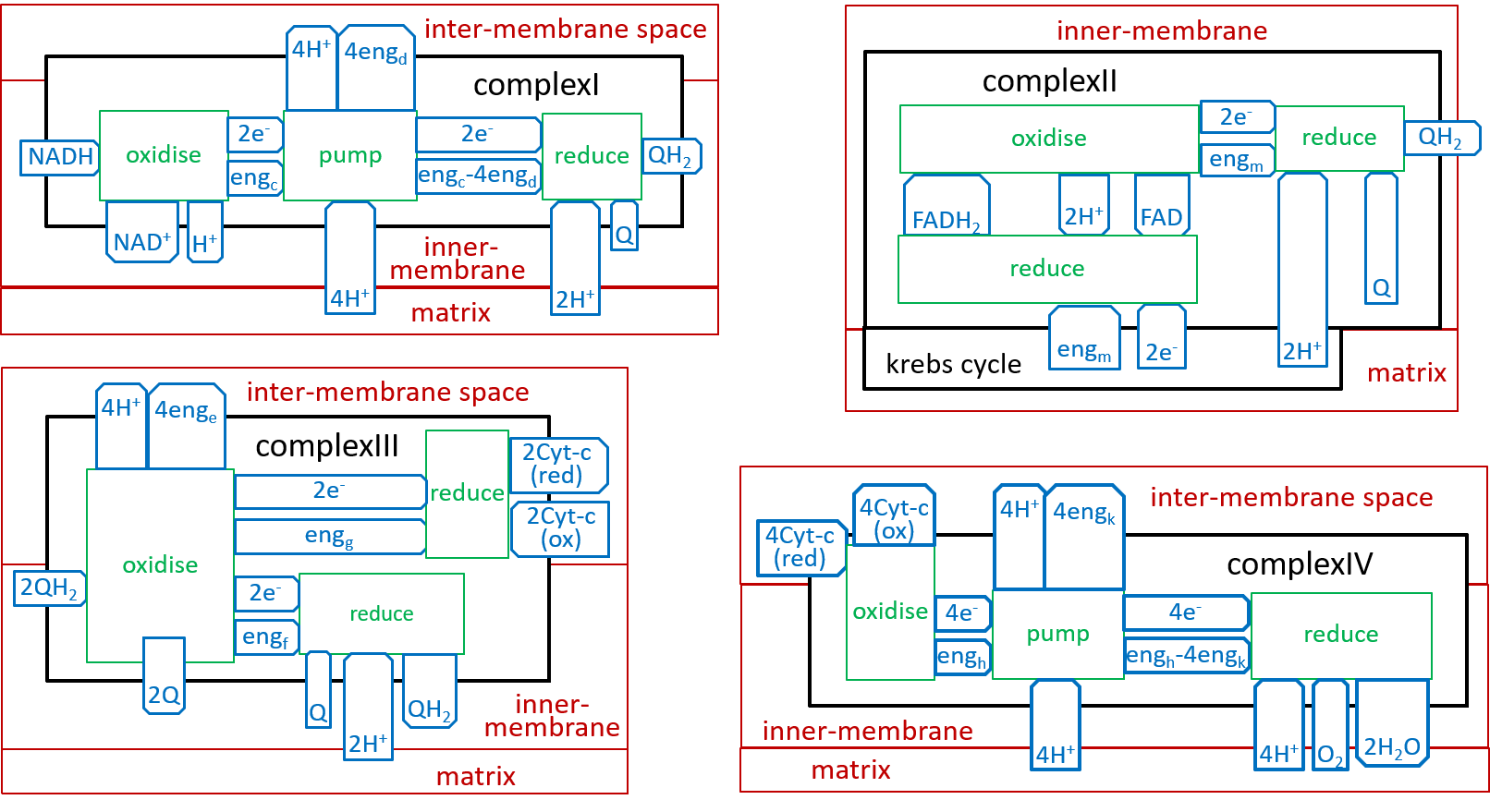
We can now develop lego-brick diagrams for the four components, of the Electron Transport Chain, as variations of the above diagram: Each electron, entering the Electron Transport Chain, is either carried, into ComplexI, within NADH, or carried, directly into ComplexII. In either case, it emerges, carried within QH₂. QH₂ then carries it, into ComplexIII, and it emerges, carried within Cyt-c(reduced). Cyt-c(reduced) carries it, into ComplexIV, and it finally emerges, carried within H₂O, water. Hence each electron, entering the Electron Transport Chain, either passes, through the sequence CompexI – ComplexIII – ComplexIV, or through the sequence CompexII – ComplexIII – ComplexIV.

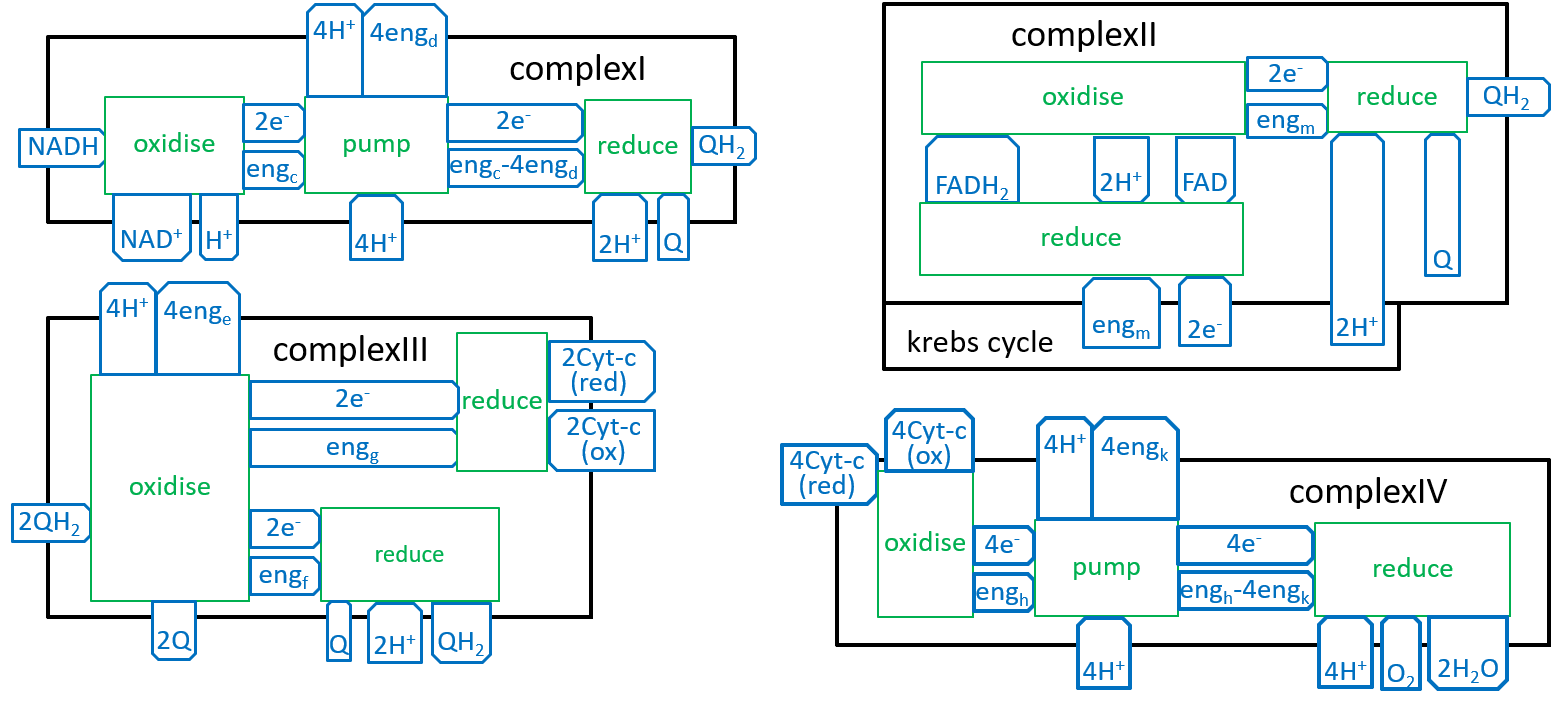
We should not think, of the Complex systems. in the above sequences, as being locked together. The Inner-Membrane contains many copies, of each, of the Complexes. As we have shown above, the electrons are carried, out, of one Complex, and into the next Complex, in its sequence, by NADH, FADH, QH₂, Cyt-c(red), or H₂O. There may be a number, of QH₂s (a pool of QH₂s), waiting to be picked up, by a ComplexIII. Eventually, each of them will be accepted by a ComplexIII. Similarly, there will be pools of NADH, FADH, and Cyt-c(red) waiting for the appropriate Complexes.

The four Complexes and their resource pools can be plugged together:: to give the full Electron Transport Chain.

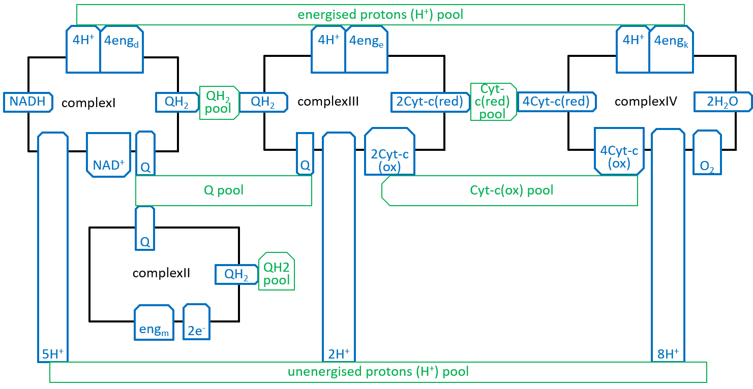
The energised proton pool is the excess of protons and energy, held in the inter-membrane space, relative to those, held in the matrix. The balance, between the electron transport chain and the atp synthesis systems, will keep the number of protons and the amount of energy, held in the pool, quite close to stability. The energy, in the energised proton pool (fed by end_d, eng_e and eng_k), will have three component parts:

electrical energy – each of the excess protons carries a charge

chemical energy – diffusion energy from the excess protons

heat energy – a small amount of spare energy, so far insufficient to pump a further proton

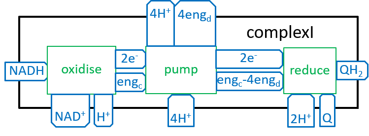
In an earlier diagram we provided a context for the Electron Transport Chain: We have yet to relate the diagrams, of this section, to that context. We can do this, by decorating each, of the four Complex diagrams, with the context:

The diagram for Complex1, presented earlier was a static view of the structure of a ComplexI system – it combined all states of the ComplexI. We should now try to represent the dynamic changes in ComplexI structure. Similar representations could be provided for ComplexII, ComplexIII and ComplexIV. A dynamic view is given by:

cx1₀( cx1₀{ α:ox, β:pp, γ:rc }, δ:NADH )

= cx1₁{ α{ δ }, β, γ }

cx1₁( cx1₁{ α:ox{ NADH{ ε:NAD⁺, ζ:H⁺, η:2e^-, θ:eng_c } }, β:pp, γ:rc }, κ:4H⁺ )

= cx1₂{ α{ ε, ζ, η, θ }, β{ η, θ, κ }, γ }

cx1₂( cx1₂{ α:ox{ NAD⁺, H⁺, η:2e^-, θ:eng_c }, β:pp{ η, θ, κ:4H⁺ }, γ:rc }, λ:2H⁺, μ:Q )

= cx1₃{ α{ }, β{ κ, ζ:4eng_d, η, π:eng_c-4eng_d }, γ{ η, π, λ, μ } }

cx1₃( cx1₃{ α:ox, β:pp{ 4H⁺, 4eng_d, η:2e^-, π:eng_c-4eng_d }, γ:rc{ η, π, λ:2H⁺, μ:Q } } )

= cx1₄{ α, β{ }, γ{ τ:QH₂{ λ, μ } } }

cx1₄( cx1₄{ α:ox, β:pp, γ:rc{ τ:QH₂ } } )

= cx1₀{ α, β, γ{ } }

ece=electro-chemical-energy epf=energised-proton-flow crg=c-ring kef=kinetic-energy-flow pfl=proton-flow

H⁺=proton cr=c-ring-subunit ke=kinetic-energy

cx1₄( cx1₃( cx1₂( cx1₁( cx1₀( cx1₀{ α:ox, β:pp, γ:rc }, NADH{ δ:NAD⁺, ε:H⁺, ζ:2e^-, eng_c{ η:4eng_d, θ:eng_c-4eng_d } } ), κ:4H⁺ ), λ:2H⁺, μ:Q ) ) )

= { cx1₀{ α, β, γ }, δ, ε, κ, η, QH₂{ λ, μ } }

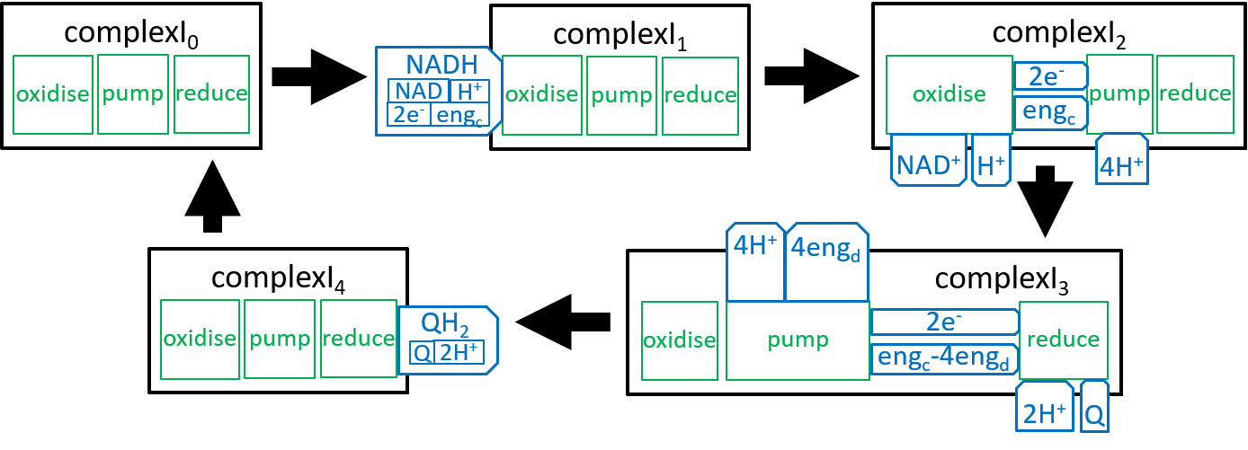
or if the composite function cx1₄( cx1₃( cx1₂( cx1₁( cx1₀( ) ) ) ) is treated as one function:

cx1( α:cx1₀, NADH{ β:NAD⁺, γ:H⁺, 2e^-, eng_c{ δ:4eng_d, ε:eng_c-4eng_d } }, ζ:4H⁺, η:2H⁺, θ:Q )

= { α, β, γ, ζ, δ, QH₂{ η, θ, ε } }

Translocators

Earlier diagrams have shown the Translocators with: We can now expand this to give: There are two translocators, one responsible for the flow of inorganic phosphate (Pi). to the matrix, and the other for the swapping of ADP and ATP molecules.

The first transporter allows a proton to move down its energy gradient, from the inter-membrane space, to the matrix. The electro-chemical energy, released by this movement, opens a channel that allows a phosphate molecule, to make the same journey. Remember that we said that an average of 3.33 protons needed to release their electro-chemical energy, during ATP synthesis. The additional energy, required by the phosphate-transporter, considered here, means that an average of 4.33 protons, in total, need to release their energy, during the formation of each ATP molecule.

The second transporter swaps ATP and ADP molecules. It moves an ADP molecule, from the inter-membrane space, to the matrix, and then moves an ATP molecule, in the opposite direction. The movement of the ADP molecule unlocks a channel, for the ATP molecule, and vice versa. Thus, this transporter cycles through two states, one state where it can transfer an ADP molecule and the other where it can transfer an ATP molecule. The swapping of ADP and ATP result in some weakening of the electro-chemical energy gradient, between inter-membrane space and the matrix.

The Krebs Cycle

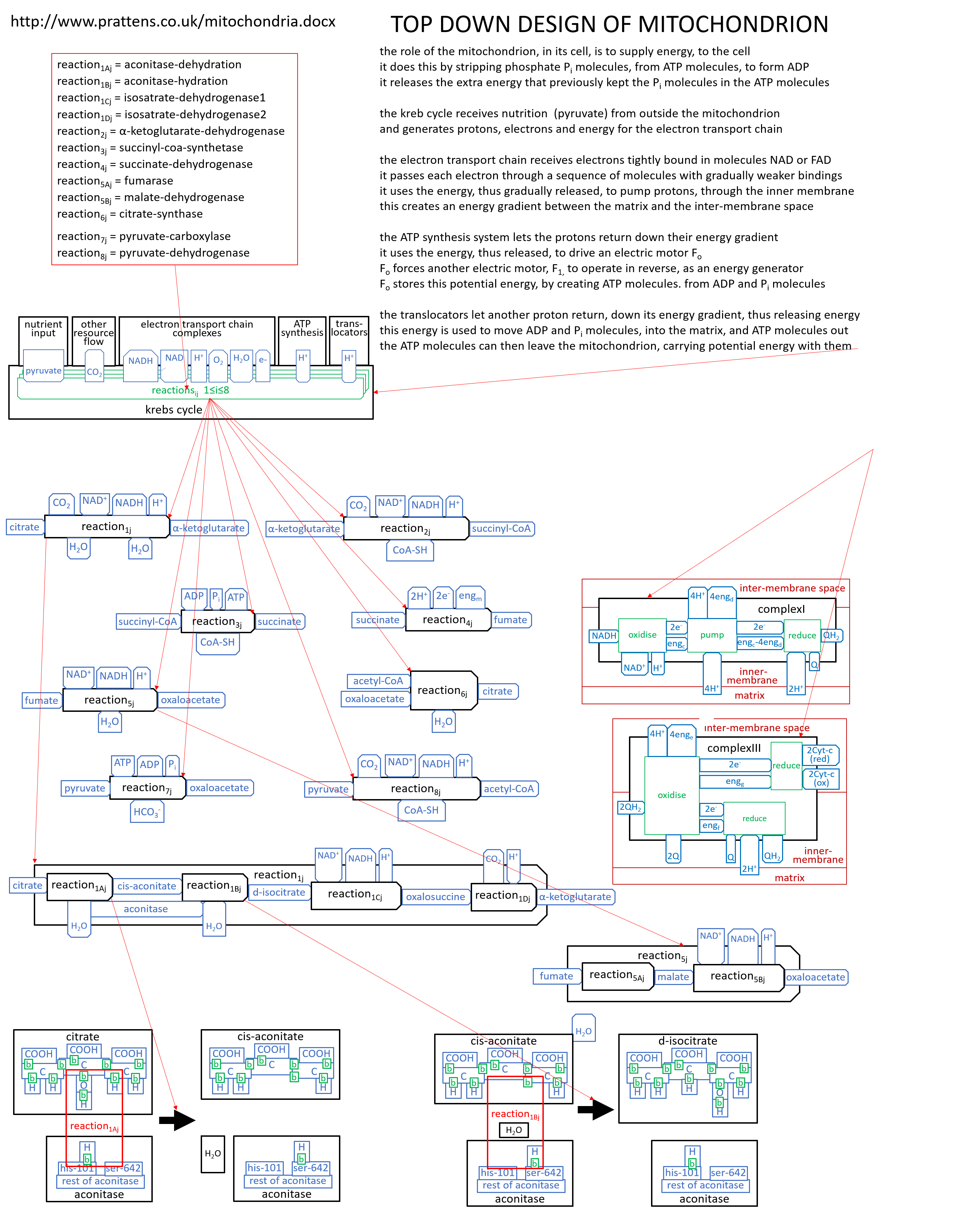
The main function, of the Krebs Cycle (or Citric Acid Cycle or TriCarboxylic Acid Cycle), is to take in the “food” that is received, by the mitochondrion, and to generate the protons and electrons that are required, by the Electron Transport Chain.

Earlier diagrams have shown how the Krebs Cycle component, of the Mitochondrion system, interacts with other components, particularly the Electron Transport Chain: There are also interactions, with the Nutrient Input and Other Resource Flow components: In this section we will consider the eight components (reactions_ij 1≤i≤8) of the Krebs Cycle system, that participate in the interactions, referred to above: The eight components are here labelled reactions_ij, with 1≤i≤8. There are multiple copies of each component, hence the label j. Remember that, earlier, we noted that the number of protons, in the Krebs Cycle system, was significant, because it determined the strength, of the proton gradient, in the ATP Synthesis and Electron Transport Chain components - hence, the label n in Krebs Cycle_n.

The eight components, of the Krebs Cycle, can be represented with the following diagrams: The top six components provide the main path of Krebs Cycle system. They show why the system is called a cycle – each component has an interaction, on its right, that matches with the interaction, on the left, of the next component – the interaction represents one component releasing a chemical and the next one picking it up, possibly after some delay. The seventh and eighth components feed the main path.

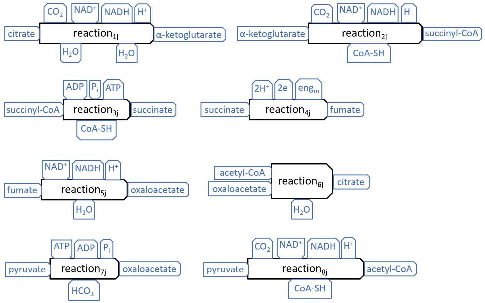
The interactions, at the top of the first five components (and the eighth), match those shown earlier, for the Electron Transport Chain and Other Resource Flow systems. The interactions, at the top of the seventh component, are the mirror image of those, on the third, so they represent a possible connection, between these components.

The other interactions shown above, except H₂O and HCO₃^- are all internal to the Krebs Cycle. The H₂O interactions represent the release of water molecules. Water can flow freely within and beyond the mitochondrion, so the water molecules may be picked up by systems, inside or outside the mitochondrion. The HCO₃^- interaction represents reaction_7j picking up a bicarbonate molecule. This molecule will have previously been created, by a reaction, between CO₂ and H₂O.

We have shown just eight reactions, because these reactions interact, in obvious ways, with each other and with the other components, of the mitochondrion, However, in most descriptions of the Krebs Cycle, two of the reactions, shown above, are broken down into subsidiary reactions, as shown below: Thus the Krebs Cycle, as usually represented, has ten components, in its main loop, plus the two that feed the loop. The chemists have given names to these twelve components:

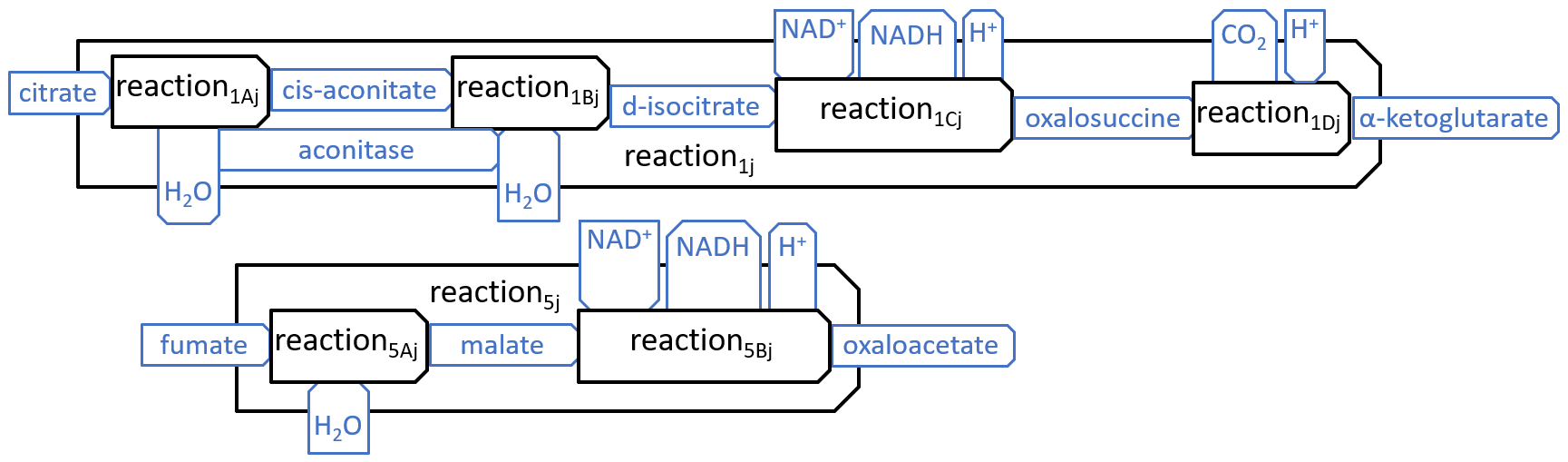
	reaction1Aj = aconitase-dehydration		reaction1Bj = aconitase-hydration
	reaction1Cj = isosatrate-dehydrogenase1		reaction1Dj = isosatrate-dehydrogenase2
	reaction2j = a-ketoglutarate-dehydrogenase		reaction3j = succinyl-coa-synthetase
	reaction4j = succinate-dehydrogenase		reaction5Aj = fumarase
	reaction5Bj = malate-dehydrogenase		reaction6j = citrate-synthase

reaction7j = pyruvate-carboxylase

reaction8j = pyruvate-dehydrogenase

or, sometimes, slight variants of these names.

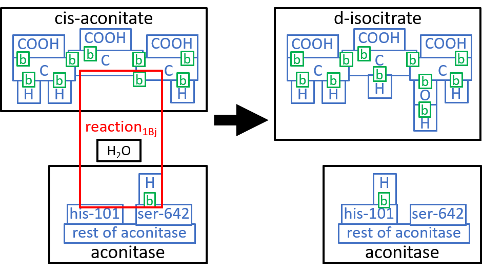
We could take these components down to the next level of detail. We will do that, here, for the first component, reaction_1Aj. The Aconitase molecule acts, as catalyst, for this reaction and the next one, reaction_1Bj. The His-101 component, of Aconitase, takes a hydroxyl group (HO), from the Citrate molecule, combines it with a proton, and thus forms an H₂O molecule. The Ser-642 component, of the Aconitase molecule, takes another proton from Citrate. These two actions result in cis-Aconitase. The next reaction, reaction_1Bj, reverses the above two actions, with His-101 and Ser-642 reversing each other’s actions. Before reaction_1Bj, the cis-Aconitase is reoriented relative to the Aconitase molecule, so that the positions of the hydroxyl group and the proton are swapped, thus forming D-Isocitrate. We can represent this with:

b=bonding

Consolidated Diagrams

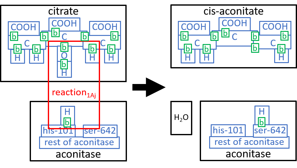
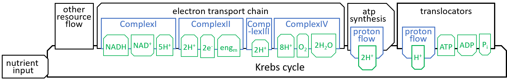
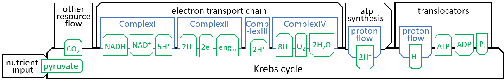
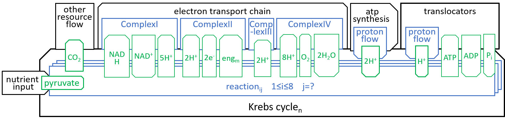
We can put the lego-brick diagrams, of the previous sections, together in one diagram. At A4 size this is:

Our Mitochondrial Model and the Viable System Model (VSM)

The previous sections have only considered a mitochondrion, when it is behaving normally. We need to add other components and systems to deal with abnormal behaviour. During the Second World War and afterwards Stafford Beer developed his Viable System Model. This model is now used widely by people developing IT systems and Business Systems.

A viable system is any system organised in such a way as to meet the demands of surviving in the changing environment.